Tuning a servo system is a complex and iterative process. It typically requires tuning multiple control loops, each with its own gains (proportional, integral, and/or derivative) to be adjusted, not to mention additional parameters such as acceleration and velocity feed-forward gains and filters to reduce oscillations.

While manual tuning has been the predominant method for many years, most servo drives now incorporate functions that will automatically tune the system. Although in the beginning, auto tuning functions were useful only when the load was rigidly coupled and the system dynamics were relatively simple, more complex algorithms and faster computing power have enabled the development of auto tuning functions that are sophisticated enough to address even the most complex systems, with minimal input or effort from the user.

Auto tuning is based on the same principles as manual tuning. That is, the performance of the motor is evaluated relative to a given command, and the servo drive automatically adjusts the gains until values are found that give the best performance. In most cases, the auto tuning process can also add filters to the control loop to suppress oscillations caused by resonance frequencies in the system.

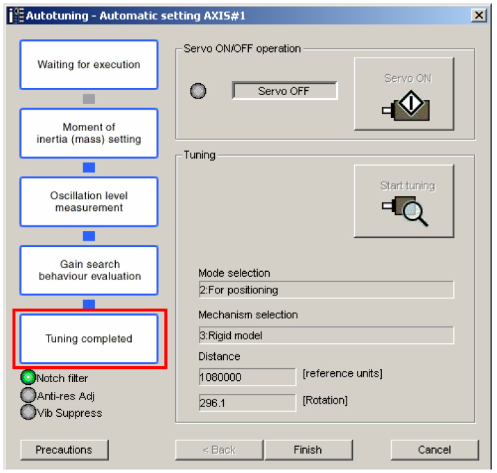
As the motor and load are driven in the auto tuning process for this Yaskawa servo drive, the drive automatically determines the inertia of the system, measures oscillations, and sets, evaluates, and optimizes the control loop gains.

Adaptive tuning is similar to auto tuning, but goes one step further and allows for a wide range of parameters that will provide stable control of the servo system. Adaptive tuning continuously monitors the system’s performance and, if necessary, adjusts the control loop gains and filter parameters to compensate for unknown or changing load conditions during the system’s operation. The key to adaptive tuning is that it runs continuously in the background of the control system to detect resonances by analyzing the frequency response of the torque loop.

One parameter tuning typically refers to a tuning feature that can be used to “fine tune” the system’s response after adaptive tuning has been configured. The term “one parameter” tuning comes from the fact that a single parameter is used to configure multiple system attributes, including gains, filters, friction compensation, and control of resonance. This improves the responsiveness, stability, overshoot, and overall efficiency of the system.

To see (and hear) a linear system with poor servo tuning, and how it can be corrected with a simple auto tuning procedure, check out this video from Bosch Rexroth.

Feature image credit: Performance Motion Devices, Inc.