Understanding vibration analysis starts with understanding the simple mass-spring-damper model shown in Figure 1, where m is the mass, k is the spring constant, c is the damping coefficient, x represents the displacement from equilibrium and f defines the force acting on the mass as a function of time. It also helps to understand some simple equations (Table 1) that describe the motion of this system and define some key parameters.
To understand why a vibration test engineer cares about these parameters, let’s look at the transmissibility plot shown in Figure 2. Transmissibility looks at how a SDOF system responds to a base excitation with a given damping and natural frequency. When the excitation frequency is much larger than the system’s natural frequency, the system isolates that base vibration. When the system’s natural frequency is much larger than the base excitation frequency, the system will neither amplify nor dampen an input vibration. The worst-case scenario is when the input frequency is equal to the system’s natural frequency, which will amplify that input by a factor approximately equal to Q.
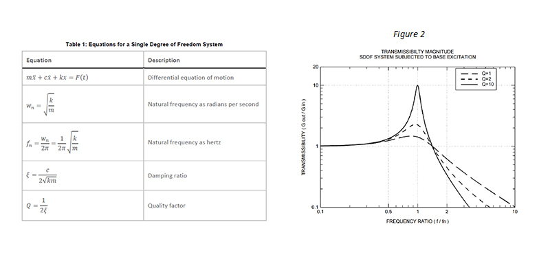
Table 1: Equations, Figure 2: The transmissibility illustrates how a SDOF system will respond to a base excitation
Most systems in the real world can’t be represented by a SDOF system, but every structure, no matter how complex, can be factored down to individual SDOF systems. And most real-world excitations are not perfect sine waves but rather a collection of sine waves. Nevertheless, vibration analysis can be used to predict how a system will react to a given input and gives engineers the tools needed to ensure the survivability of their systems. Vibration testing allows them to understand the vibration environment.
Simple Analysis in the Time Domain
When analyzing vibration data in the time domain (amplitude plotted against time), we’re limited to a few parameters in quantifying the strength of a vibration profile: amplitude, peak-to-peak value, and RMS. Figure 3 shows a simple sine wave with these parameters identified.
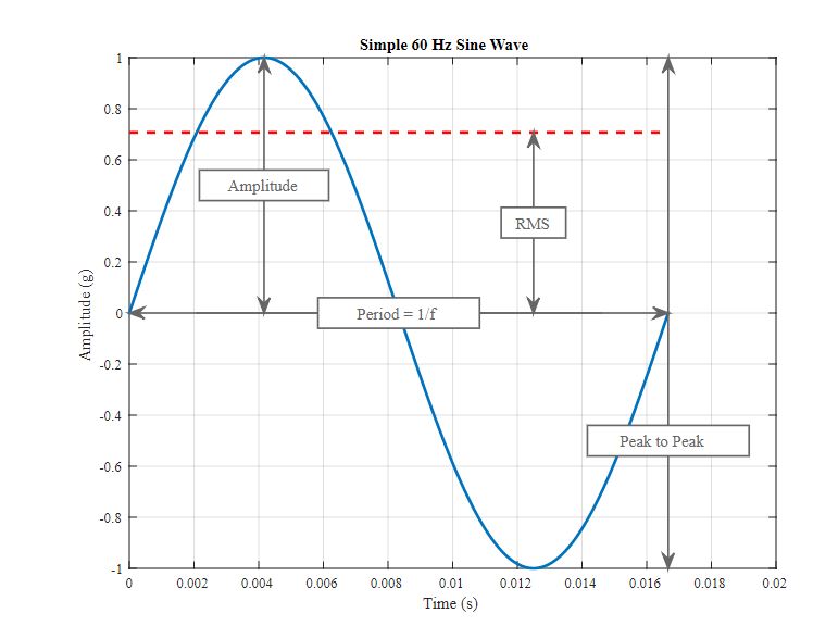
Figure 3: A simple 60 Hz sine wave with the amplitude, peak-to-peak, RMS, frequency, and period identified.
- The peak or amplitude is valuable for shock events, but it doesn’t take the time duration and therefore the energy in the event into account.
- The same is true for peak-to-peak with the added benefit of providing the maximum excursion of the wave, which is useful when looking at displacement information, specifically clearances.
- The RMS (root mean square) value is generally the most useful because it is directly related to the energy content of the vibration profile and therefore the destructive capability of the vibration. RMS also takes into account the time history of the waveform.
Vibration is an oscillating motion about equilibrium, so most vibration analysis looks to determine the rate of that oscillation, or the frequency that is proportional to the system’s stiffness. The number of times a complete motion cycle occurs during a period of one second is the vibration’s frequency and is measured in hertz (Hz). For simple sine waves, the vibration frequency could be determined by looking at the waveform in the time domain, but as different frequency components and noise are added, spectrum analysis is necessary to get a clearer picture of the vibration frequency.
Fast Fourier Transform (FFT)
Any waveform is actually just the sum of a series of simple sinusoids of different frequencies, amplitudes, and phases. A Fourier series is that summation of sine waves; we use Fourier analysis or spectrum analysis to deconstruct a signal into its individual sine wave components. The result is acceleration/vibration amplitude as a function of frequency, which allows performing analysis in the frequency domain (or spectrum) to gain a deeper understanding of the vibration profile. Most vibration analysis will typically be done in the frequency domain.
A discrete Fourier transform (DFT) computes the spectrum, but nowadays this has become synonymous with the fast Fourier transform (FFT), which is just an efficient algorithm for the DFT.
The most important thing to understand is that the number of discrete frequencies that are tested as part of a Fourier transform is directly proportional to the number of samples in the original waveform. With N being the length of the signal, the number of frequency lines or bins is equal to N/2. These frequency bins occur at intervals (Δf) equal to the sample rate of the raw waveform (Fs) divided by the number of samples (N), which is another way of saying that the frequency resolution is equal to the inverse of the total acquisition time (T). To improve the frequency resolution, it’s necessary to extend the recording time.
Δf=1T=FsN
The lowest frequency tested is 0 Hz, the DC component; the highest frequency is the Nyquist frequency (Fs/2).
Constructed Sine Wave and FFT Example
To illustrate how an FFT can be used, let’s build a simple waveform with three different frequency components: 22 Hz, 60 Hz, and 100 Hz. These frequencies will have amplitudes of 1g, 2g, and 1.5g respectively. Figure 4 shows how this waveform looks a little confusing in the time domain and also illustrates how the signal length affects the frequency resolution of the FFT.
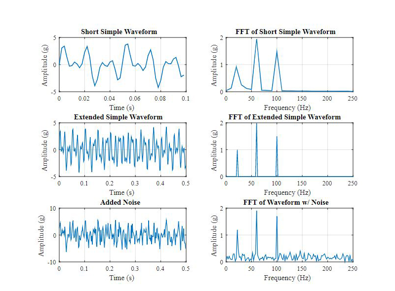
Figure 4: Constructed waveform with 22, 60, and 100 Hz frequency components at varying sample lengths and with noise to illustrate the usefulness of FFT analysis.
If this wave is sampled at 500 Hz (500 samples per second) and an FFT of the first 50 samples is taken, the result is a pretty jagged FFT because the bin width is 10 Hz (Fs of 500 divided by N of 50). The amplitudes of these frequency components are also a bit low. But if the range is extended to the first 250 samples (middle row), then the FFT can calculate both the frequency and amplitude of the individual sine wave components accurately. If broadband noise is added as shown in the bottom row, then the waveform becomes even less distinguishable. This is the power of an FFT; it can clearly identify the major frequencies that exist to help the analyzer determine the cause of any vibration signal.
Windowing
Fourier transforms perform an integral from negative infinity to positive infinity, but data can only be acquired over a discrete time period. So a Fourier transform must repeat the signal infinitely to perform the transform. When the acquired data begins and ends at 0, or if there are an integer number of cycles, then this infinite repetition will cause no problems. But if these are not true, there will be leakage in the frequency domain because the signal is distorted, as shown in Figure 5.
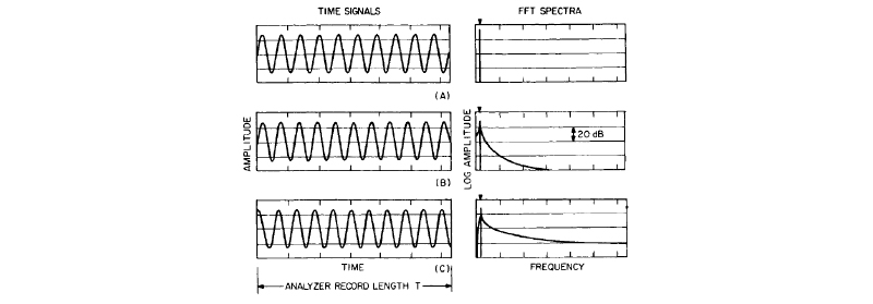
Figure 5: The time-window effects are shown when using a FFT analyzer without windowing (or rather a uniform window) are shown. (A) represents an integer number of cycles so that the spectrum has a clear spectral line. (B) and (C) represent time signals where there are a half-integer number of periods, but with different phase relationships, which gives a different discontinuity and spectral leakage.
Remember that a Fourier transform looks to calculate a series of sine waves to represent the data. If there is a discontinuity in the data (by not beginning and ending at 0 or not having an integer number of cycles), then the FFT analyzer will need many terms to approximate the apparently discontinuous signal.
To minimize this error, windows are used to better make the signal appear periodic for the FFT process. The most common windows are the rectangular window, the Hanning window, the flattop, and the force/exponential window (used for impact testing). All windows distort the data; although, they are sometimes necessary, they aren’t always required if the vibration tester can satisfy Fourier’s request by completely observing the signal in one sample of data.
Spectrogram and FFT Comparison
Real-world applications typically have many different frequency components in their vibration profile, as well as mechanical and electrical noise. Figure 6 shows some data from a idling car engine that was taken with a Slam Stick vibration data logger.
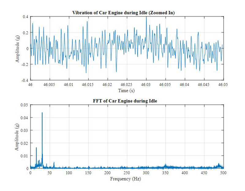
Figure 6: A car’s engine during idle clearly shows the 30 Hz dominant frequency, which equals twice the crankshaft rotation frequency of 15 Hz (900 RPM) where a peak is also visible.
Car Engine Spectrum Analysis
Spectrum analysis of the vibration profile can indicate the crankshaft rotation speed of this 4-cylinder, 4-cycle engine. The engine operates with two pairs of pistons moving out of phase with each other and two piston combustions per crankshaft rotation, so the dominant frequency of the engine’s vibration will be twice the crankshaft rotation speed. The FFT shows a dominant frequency at 30 Hz or 1,800 RPM, which indicates that, at idle, the crankshaft is rotating at 900 RPM (or 15 Hz) where there is also a peak in the FFT. The use of an FFT in our vibration analysis gave clues on what was causing the measured vibration.
In many applications, the vibration frequency changes over, so examining the FFT is not enough. Figure 7 shows the vibration when the engine is running at a relatively fixed rate and an FFT of the entire signal. In this test, the engine was turned off for a period, idled, then revved before being allowed to idle again and finally turned off. Although the vibration frequency changed pretty dramatically throughout the test, the FFT doesn’t capture that. Figure 6 showed that when the engine was idling, there was a fairly significant dominant vibration frequency of 30 Hz, but this peak gets muted when looking at the FFT of a changing vibration environment.
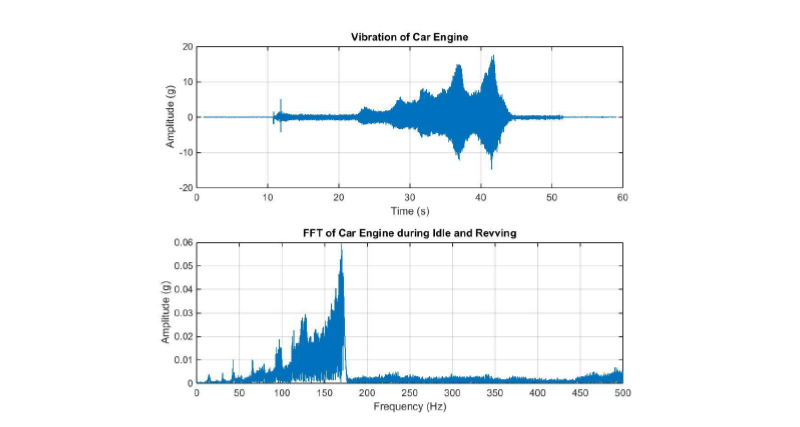
Figure 7: The time history and FFT are shown from a Slam Stick mounted to an engine block while it was revved to change the dominant frequencies.
A spectrogram is needed in applications where the vibration frequency changes with time. A spectrogram works by breaking the time domain data into a series of chunks and taking the FFT of these time periods. These series of FFTs are then overlapped to visualize how both the amplitude and frequency of the vibration signal change with time. Turn this 3D surface plot of FFTs on its side, add a color scale to represent the amplitude (often works best when visualizing the color/amplitude on a logarithmic scale) and the result is a spectrogram.
Figure 8 illustrates how the dominant frequencies change with time in relation to when the car engine was idled and revved. Using a spectrogram allows gaining a much deeper understanding of the vibration profile and how it changes with time.
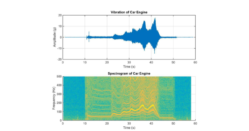
Figure 8: Spectrogram of engine shows how crankshaft speed change (when engine is revved) affects vibration frequencies.
Power Spectral Density (PSD)
A lot of real-world vibration is considered “random” because it occurs at many frequencies simultaneously. Although FFTs are great at analyzing vibration when there are a finite number of dominant frequency components, power spectral densities (PSD) are used to characterize random vibration signals. A PSD is computed by multiplying each frequency bin in an FFT by its complex conjugate, which results in the real only spectrum of amplitude in g2. The key aspect of a PSD that makes it more useful than a FFT for random vibration analysis is that this amplitude value is then normalized to the frequency bin width to get units of g2/Hz. Normalizing the result eliminates the dependency on bin width, allowing for comparison of vibration levels in signals of different lengths.
PSDs are powerful because the area under the curve (or integral) in the frequency domain represents the RMS vibration level for that frequency range. And RMS vibration is related to the energy in the environment. PSDs are also often used in test standards because of how they cancel out the effect of bandwidth of a frequency spectrum. For anyone buying equipment to be integrated into a larger system, it’s critical to ensure that equipment can handle the vibration levels in this environment so we may require a test organization to quantify that environment. Recently, a Slam Stick was used to record vibration data on a commercial flight (Figure 9) to understand the levels of vibration humans were exposed to during flight.
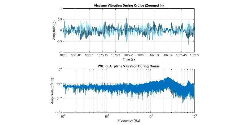
Figure 9: Random vibration levels on the seat of a commercial airliner.
There is definitely a resonance of that seat around 250 Hz, but there is surprisingly steady broadband vibration of 10-5 g2/Hz from 1 Hz to 1 kHz. This PSD could be used to program an exposure profile in a laboratory shaker to allow performing some in-house testing ahead of a field test. Because this was from actual data in the actual environment, the engineering team can be confident that their system can survive.
Steve Hanly is Vice President of Sales and Marketing for Midé Technology Corporation. He joined the company as an engineer in 2010 and has since held a number of engineering, product management and marketing positions with the company. Hanly holds an undergraduate and master’s degree in mechanical engineering and aerospace engineering, both from Worcester Polytechnic Institute, and is currently in an MBA program from University of Massachusetts, Amherst.
Filed Under: Product design