The radar sitting in your car’s bumper isn’t the same as the units vectoring planes in for a landing. Here are the most important differences.
Leland Teschler | Executive Editor
The last time you found yourself on an airplane, it’s likely that air traffic controllers kept track of you via radar sets operating at about 2 GHz. In contrast, the radar that helps park your car and keeps you from hitting vehicles braking hard in front of you pumps out signals at 77 GHz. (Older systems used 24 GHz, to be phased out by 2022.)
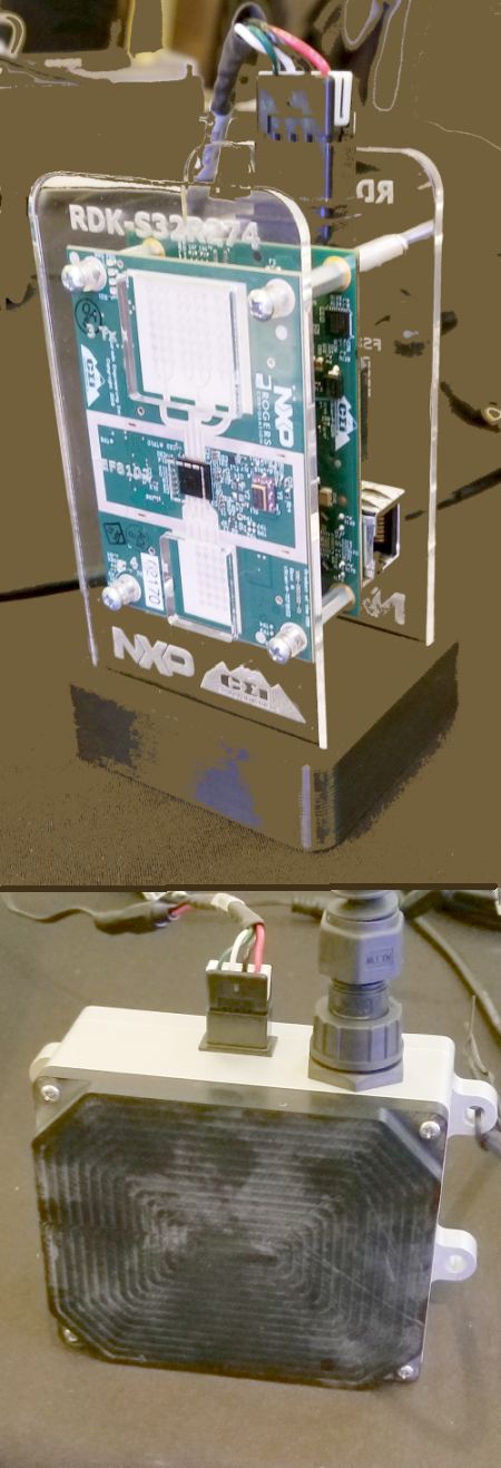
Automotive radar today often takes the form of a module containing an RF board and a signal processing board. An example is the RDK-S32R274 module from NXP. It typically serves as a radar development platform but can also be used as-is for such tasks as collision avoidance, adaptive cruise control, and occupancy detection. Visible here is the TEF8102 RFCMOS transceiver and antenna arrays. An S32R27 microcontroller and FS8410 Power Management IC sit on the board mounted behind the RF section. Maximum range is said to be 180 m with a range accuracy of 0.175 m. Angular resolution is said to be 4.25° ±0.25°. Bottom, an enclosed automotive radar module with its antenna toward the camera.
There are several kinds of radar in wide use today. The type employed in vehicles is called frequency modulated continuous wave, FMCW. (There is academic work on OFDM and random radar, but these types need more processing power than is currently practical.) Rather than send out a simple pulse that reflects back from targets, FMCW sends out a chirp, a pulse whose frequency rises during its transmission. The difference between the frequency of the chirp coming out of the transmitter and the frequency of the received reflection (at any one time) is linearly related to the distance from the transmitter to the object.
The current generation of radar-equipped vehicles typically has one front radar for adaptive cruise control with about a 150-m range. There is often a second front radar with a wider field of view (FOV) for emergency brake assist. In the rear, there are two radars with up to an 80-m range for detecting vehicles behind the car.
Industry analysts expect the range of all these radars to rise in the future, especially for rear radar which is forecast to reach 160 m. The overall effect will be that of a 360° cocoon around the car.
Building blocks
The typical vehicular radar module today contains five major functional building blocks: The antenna, the RF section, a high-speed digital interface, a signal processor, and a power section.
Automotive systems have two types of antennas, vertical and horizontal polarization, or just V and H. V is the traditional type. Vertical polarization has the benefit of less clutter but a limited azimuth (angle of horizontal deviation) FOV because the single-element patch V radiator has a narrow radiation pattern. Similarly, horizontal polarization entails a wider azimuth FOV but more ripples in the resulting pattern of targets.
Most radar front-end components employ RF CMOS. The usual configuration is to put RF components on one PCB, signal processing on another. (It’s possible to find single-chip radar units, but because both the processor and RF components run hot, there can be thermal challenges.)
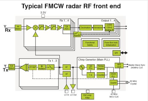
A block diagram of an MR3003 transceiver chip from NXP illustrates the typical makeup of an automotive FMCW module. A local oscillator (LO) generates a linear frequency-modulated continuous wave signal, the chirp, which is amplified by a power amp and transmitted from the antenna. The receive antenna intercepts the reflected signal which is then amplified and mixed with the LO signal. This mixing produces the sum of the LO and echo frequencies and their difference. The sum is filtered out and the difference (the beat-frequency or intermediate-frequency, IF) output is then sent to a processing module where it is digitized.
In a typical automotive FMCW module, a local oscillator (LO) generates a linear frequency-modulated continuous wave signal, the chirp, which is amplified by a power amp and transmitted from the antenna. The receive antenna intercepts the reflected signal which is then amplified and mixed with the LO signal. This mixing produces the sum of the LO and echo frequencies and their difference. The sum is filtered out and the difference (the beat-frequency or intermediate-frequency, IF) output is digitized. The digitized output of the ADC goes to a signal processor that analyzes the resulting signals for targets. The signal processor typically incorporates between two and six cores and includes dedicated hardware for FFTs.
A point to note is that the interface to other automotive subsystems tends to be a serious limiting factor for radar systems. To see why, consider that one radar sensor samples at an effective rate of 20 MS/sec over a 10 msec measurement time with a 50-msec cycle time. If the ADC is at 12 bits/sample, a quick calculation gives 1.2 MB per measurement and a 24 MB/sec data rate for four receive channels. The problem is that fastest pipe today is high-speed Ethernet. Its bit rate is 100 Mbit/sec or only 11.75 MB/sec. Thus, if used with a radar sensor, a high-speed Ethernet connection would have sensor data backing up at the rate of 12.25 MB/sec.
Auto radar today typically uses a chirp waveform with frequency increasing from 77 to 77.8 GHz. The instantaneous difference in frequency between the transmitted and echoed signals is directly proportional to the time delay, and time delay is directly proportional to the range. Thus, a measurement of the IF signal gives range information. A digitized version of it is the basis for calculating range and identifying targets.
A complication arises when the targets are moving. There is a shift in the frequency of the reflected wave because of the Doppler effect, so the IF frequency depends not only on the range but also on the relative velocity of the target. To resolve the ambiguity, auto radars typically use their signal processor to separate the Doppler frequencies from the range frequencies.
The usual technique is to emit several fast chirps, i.e. a chirp sequence. The resulting data gets put in a data matrix that is often represented as a two-dimensional array, with the detected frequencies of each collected chirp shown in a single column.
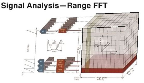
Auto radars typically use their signal processor to separate the Doppler frequencies from the range frequencies. The usual technique is to emit several fast chirps, then put the resulting echo data in a matrix that is often represented as a two-dimensional array, with the detected frequencies of each collected chirp shown in a single column. The contents of the columns are generally dubbed “fast time” whereas the contents of the rows are called “slow time.” An FFT performed on the fast-time entries followed by an FFT on the slow-time data gives a speed and a range for one or more targets. Automotive applications also need to resolve targets in terms of their angular position from the radar sensor. To do so, radars generally employ between four and 16 antennas. A fast and slow-time FFT takes place on each antenna output. The resulting data is often visualized as a cube with X and Y axes composed of the fast and slow-time data and a Z axis representing the data for each of the antennas. Effectively, this cube represents a 3D map with axes of speed, distance, and azimuth.
The contents of the columns are generally dubbed “fast time” whereas the contents of the rows are called “slow time.” Chirp-sequence signal processing starts with an FFT performed on the fast-time entries followed by an FFT on the slow-time data. An FFT along the fast time axis effectively provides what’s called a range compression because it compresses all the reflected energy into a range. Similarly, the second FFT along the slow-time axis provides a speed compression. In the simple case where there is a single target, get a single peak at the target’s range and velocity.
The two-dimensional FFTs give a speed and a range for one or more targets. The targets are basically peaks above some noise threshold. (The setting of this threshold is a processing problem in and of itself.) But automotive applications also need to resolve targets in terms of their angular position from the radar sensor. To measure this angular position, radars employ multiple antennas, generally between four and 16. A fast and slow-time FFT takes place on each antenna output. The resulting data is often visualized as a cube with X and Y axes composed of the fast and slow-time data and a Z axis representing the data for each of the antennas. Effectively, this cube represents a 3D map with axes of speed, distance, and azimuth.
The angular position of the target is determined by the amplitude ratio of the received signals in adjacent radar beams, typically referred to as a monopulse technique. Monopulse techniques send out radar signals in slightly different directions (and perhaps slightly different phases). The reflected signals are amplified separately and compared to each other, indicating which direction has a stronger return, and thus the general direction of a target relative to the radar’s main axis. This comparison takes place during one pulse, hence the monopulse moniker.
The benefit of the monopulse method is that it is computationally cheap — it can easily track 100 targets in each measurement cycle. One drawback is a relatively rough angular resolution. So, radar system signal processors typically apply a quick test to each echo they discern to decide whether it is from a single target or from several that must be separated. The separation process entails use of more sophisticated algorithms such as Bartlett or MVDR (minimum variance distortionless response) beamforming.
The bigger the effective receiving cross-section (aperture) of the antenna, the greater the ability to resolve the angle of targets. That is why there is great interest in fielding MIMO (multiple in/multiple out) antenna arrays for automotive radar. A MIMO array having just four receive channels and three transmit channels can synthesize an array of 12 virtual receive antennas with a commensurate rise in antenna aperture.
All in all, chirp-sequence FMCW radar in automotive applications typically can resolve the range of targets to between 7 and 36 in over a typical range of from 20 to 200 m. Range resolution is inversely dependent on chirp bandwidth; bandwidth can be 800 MHz, 1 GHz, or 1.6 GHz. Auto radars can typically resolve velocities to within the range of 0.14 to 1.14 m/sec.
A final point to note is that situational factors can greatly impact radar performance. A classic example is the metallic paint applied to bumpers. The paint covers not only the bumper but also the radar antennas used for parking. Experts say this metallic paint degrades the detection range of the radar by a factor of 1.5 to 1.7. DW
References
NXP S32R Radar Software Development Kit (SDK)
You may also like:


Filed Under: Automotive, The Robot Report, ELECTRONICS • ELECTRICAL, Microcontroller Tips